Accelerated Methods in {Multi-Modal, Multi-Metric, Many-Model} CogNeuroAI
A tutorial showcasing a number of (GPU-accelerated) methods for probing the representational alignment of brains, minds, and machines. An exploration of computational modeling methods at the intersection of cognitive neuroscience and artificial intelligence.
Introduction
An exploration of the Multi-Modal, Multi-Metric, Many-Model computational modeling methods at the intersection of cognitive neuroscience and artificial intelligence – the emerging field of NeuroAI.
Subsequent, updated versions of this tutorial will be made available via GitHub at github.com/ColinConwell/DBM-Tutorial.
Background: Understanding how the brain transforms sensory input into representations that support adaptive, real-world behavior has long been a foundational goal of cognitive neuroscience. Developed with an industrial fervor scarcely seen since the days of steel and railroad, task-performant deep neural network (DNN) models have now become a central part of the neuroscientific toolkit – not just as artifacts of engineering, but as theoretical objects whose internal representations can be mapped systematically to biological neural activity
In this tutorial, we’ll explore three of NeuroAI’s most actively expanding frontiers: the study of representational alignment between natural and artificial neural systems
The tutorial is organized (roughly) into two chapters:
-
Chapter 1: Intro to DeepJuice
An introduction to the DeepJuice library, and a reproduction of the main analysis in, which probes multiple forms of representational alignment between visual deep neural networks and ventral visual cortex activity in the widely used Natural Scenes Dataset . -
Chapter 2: Enter Now the LLM
Exploring the kinds of inferences and analysis made possible by language models, with a case study in cross-modal representational alignment, and language-specified, hypothesis-driven interpretability probes based on vector-semantic mapping with “relative representations”.
DeepJuice: High-Throughput (GPU-Accelerated) Brain & Behavioral Modeling
DeepJuice is a library for performing various kinds of readout on deep neural network models. It includes tools and functionality designed specifically for high-throughput model instrumentalization, feature extraction, dimensionality reduction, neural regression, transfer learning, manifold statistics, and mechanistic interpretability. It also includes a large collection of models (and relevant metadata) that allows for controlled experimental comparison across models that vary in theoretically interesting ways.
The Controlled Comparison Approach: A key methodological insight underlying this work is that we can conceptualize each DNN as a different “model organism” – a unique artificial visual system with performant, human-relevant visual capacities. By comparing sets of models that vary only in one factor (e.g., architecture, task, or training data) while holding other factors constant, we can experimentally examine which inductive biases lead to more or less brain-predictive representations. This approach moves beyond simply ranking models on a leaderboard, toward understanding why certain representations align better with the brain than others.
Target Brain Region: Our primary target is human occipitotemporal cortex (OTC), a broad swath of high-level ventral visual cortex encompassing category-selective regions for faces, bodies, scenes, and objects. But our interest extends beyond object recognition per se – OTC is increasingly understood as a “feature bank” whose representations support not just categorization but flexible, adaptive behavior across many tasks. The same representations that predict OTC activity may also predict human behavioral similarity judgments, generalization patterns, and semantic associations.
In this walkthrough, we demonstrate the methodology from
A reproduction of the first figure (showing an overview of the analysis pipeline) in
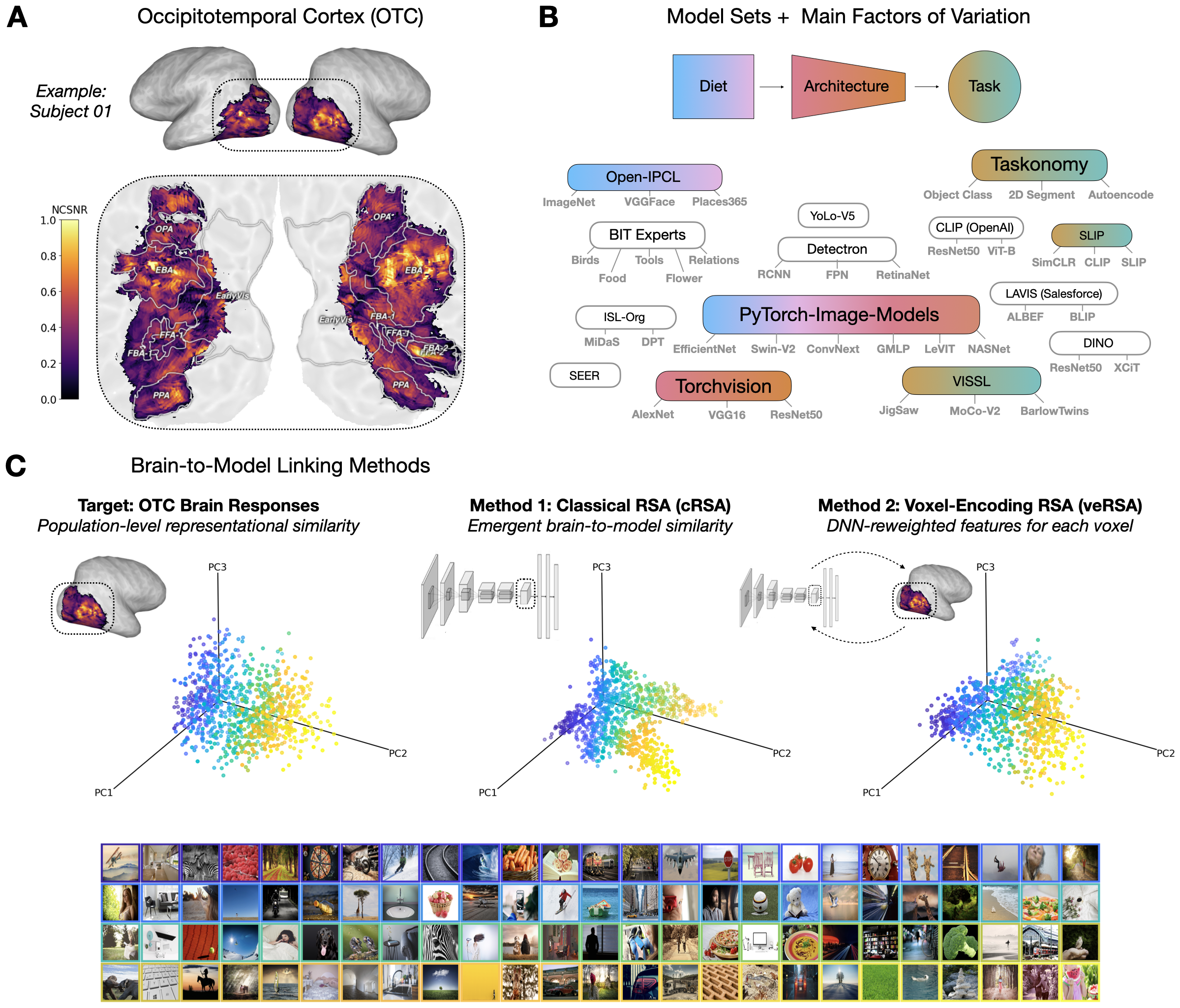
- In (A), we have an example of our target brain data: occipito-temporal cortex activity (in this case, from a single example subject, colored by a measure of reliability called NCSNR).
- In (B), we see a schematic of the underlying model repositories that power our controlled model comparison, grouped by specific axes of experimental interest with implications for the kinds of ‘representational pressures’ that could in theory have played a role in shaping the representations we read in the brain data.
- In (C), we see a schematic of our representational alignment (“linking”) procedures (classic RSA, encoding RSA – with the figure-implicit encoding models that are fit in between). More detail on all 3 of these below!
Step 0: Environment Setup
As deepjuice remains in active development, the particular setup steps may change over time. For the latest setup steps, please refer to the tutorial’s GitHub repo.
Global environment setup
```python import os, sys tutorial_repo = 'https://github.com/ColinConwell/DBM-Tutorial' notebook_path = os.getcwd() # current working directory try: # to import deepjuice, then check for local clone from deepjuice import SystemStats except ImportError as error: print('deepjuice installation not found. Checking for local clone...') DEEPJUICE_DIR = os.path.join(notebook_path, 'DeepJuice') if os.path.exists(DEEPJUICE_DIR): sys.path.insert(0, DEEPJUICE_DIR) else: # raise error directing to repo raise RuntimeError(f"deepjuice not found. Please refer to {tutorial_repo} for setup instructions.") ```Working on a shared machine with multiple GPU devices? DeepJuice at the moment works sufficiently well with a single GPU for testing purposes. In the code below, we’ll modify the global environment to only “see” a single GPU, meaning all subsequent processes will default to using this GPU. Proactively, we’ll set this to be the last available GPU in the list, so as to minimize the likelihood of conflict with concurrent processes or traffic.
GPU device selection
```python from deepjuice.systemops.devices import count_cuda_devices device_to_use = count_cuda_devices() - 1 if device_to_use >= 0: # no update if no device os.environ['CUDA_VISIBLE_DEVICES'] = str(device_to_use) ```Conceptual Primer: Representational Alignment
Before diving into the code, it is worth considering the conceptual foundations of what we are trying to measure. Representational alignment refers to the degree of correspondence between internal representations in two systems – in our case, artificial neural networks and the human brain. But how exactly should we quantify this correspondence? And what does it mean when two systems are “aligned”? A recent community effort
- How do we measure similarity between representations?
- Do similar representations lead to similar behavior?
- How can we modify representations to better align them?
This tutorial focuses primarily on the first question, while keeping the others in mind.
The Challenge of Comparison: Representations in DNNs and brains exist in different coordinate systems, with different dimensionalities, and are accessed through different measurement modalities. Any comparison requires assumptions about what aspects of representation matter. As
Two Families of Methods: In this tutorial, we explore two complementary approaches:
-
Representational Similarity Analysis (RSA): Compares the geometry of representations by asking whether stimuli that are represented as similar in the model are also represented as similar in the brain
. This approach abstracts away from individual features to focus on relational structure – the pattern of distances between stimuli. -
Encoding Models: Learns a weighted mapping from model features to brain activity, then evaluates on held-out data
. This approach allows the brain to “select” which model features are relevant, but introduces many degrees of freedom that can make even dissimilar representations appear aligned.
We will use both approaches, as well as hybrid methods (encoding RSA) that combine their strengths. The goal is not to find “the best” metric, but to understand what different metrics reveal about model-brain correspondence.
The powerhouse of all our comparisons will be DeepJuice: a single unified API that combines model zoology, feature extraction, dimensionality reduction, and alignment techniques together in a single, GPU-accelerated package, written in PyTorch, designed for cognitive scientists.
Intro: Import the Juice
To get started, let’s load all relevant deepjuice modules below:
from deepjuice import * # imports all deepjuice modules
from deepjuice.first_steps import * # tutorial helpers
Welcome to DeepJuice!
Step 1: Selecting a Model
Model Options
The first part of most DeepJuice analyses will involve loading a pretrained deep neural network model. In the DeepJuice model zoo (which we affectionally refer to as “the orchard”), you’ll find a large number of different, registered models. get_model_options() (the main function from deepjuice/model_zoo) will return a pandas dataframe of the various models we’ve already implemented. Note that while these are the models that will be easiest to use with deepjuice, almost any PyTorch model will work just as well.
# here's a sample of 5 deepjuice models from the model_zoo
get_model_options().sample(5)
The output of get_model_options() can be parsed as a regular pandas dataframe, but you can also throw various arguments in there to return specific subsets of the model zoo, by passing a dictionary of the form {metadata_column_name: search_query}. And if you just want the unique ID (uid) of the models that can be used to load them, you can ask get_model_options for a list.
# here are a sample of 5 deepjuice models from OpenCLIP
get_model_options({'source': 'openclip'}).sample(5)
# here is a list of all available OpenAI clip models in deepjuice:
get_model_options({'source': 'clip'}, output='list', exact_match=True)
['clip_rn50',
 'clip_rn101',
 'clip_rn50x4',
 'clip_rn50x16',
 'clip_rn50x64',
 'clip_vit_b_32',
 'clip_vit_b_16',
 'clip_vit_l_14',
 'clip_vit_l_14_336px']
Load the Model
Once you’ve decided on a model to use, just pass the model_uid to the following function. Crucially, this function by default will return both the pretrained model and the preprocessing function that should be applied to the data you intend to perform readout over. (Note: If using certain models – like OpenCLIP – in a Colab environment, you may be required to install the relevant packages, e.g. pip install open_clip_torch.)
For this walkthrough, we’ll be using a pretrained AlexNet model from Harvard Vision Science Laboratory’s OpenIPCL repository. This model is a self-supervised contrastive learning model trained over the images (but not the labels) of the ImageNet1K dataset.
# list all (Harvard) IPCL models available in deepjuice
get_model_options({'model_uid': 'ipcl'}, output='list')
['ipcl_alexnet_gn_imagenet1k',
 'ipcl_alexnet_gn_openimagesv6',
 'ipcl_alexnet_gn_places2',
 'ipcl_alexnet_gn_vggface2',
 'ipcl_alexnet_gn_mixedx3']
model_uid = 'ipcl_alexnet_gn_imagenet1k'
model, preprocess = get_deepjuice_model(model_uid)
Critically, almost all deepjuice functionality is predicated on the model object having a forward function that is called directly over an input tensor as follows: model(inputs). All registered models in DeepJuice have this property implicitly specified, but if you’re using a custom model, or want a variation of the function, you can always specify your own!
Step 2: Feature Extraction
You’ve now loaded a model and you want to know how the model responds to a given set of inputs – potentially at more than one stage of the model’s information-processing hierarchy. This procedure is typically called feature extraction, and involves saving the intermediate outputs of one or more of a model’s many layers.
In the example below, we’ll grab some sample images, and pass them through our loaded model, collecting both features and feature metadata as we do. This is a relatively small set of inputs, but just note that feature extraction procedures can get very computationally expensive very fast. We’ll discuss how to manage this overhead in the Memory Management subsection below.
DataSets + MetaData
from juicyfruits import get_sample_images

# let's grab a quick sample of 5 images
sample_image_paths = get_sample_images()
print('\n'.join(["   Sample image paths:", *[os.path.relpath(path, os.getcwd()) for path in sample_image_paths]]))
Initializing DeepJuice Benchmarks
   Sample image paths:
DeepJuice/juicyfruits/quick_data/image/vislab_logo.jpg
DeepJuice/juicyfruits/quick_data/image/william_james.jpg
DeepJuice/juicyfruits/quick_data/image/grace_hopper.jpg
DeepJuice/juicyfruits/quick_data/image/xaesthetics_logo.jpg
DeepJuice/juicyfruits/quick_data/image/viriginia_woolf.jpg
# let's get our dataloader now, which takes our image_paths
# and! our model preprocessing function, returning tensors
dataloader = get_data_loader(sample_image_paths, preprocess)
# let's start by getting all our model's feature maps, since we have only a small number of images:
# get_feature_maps requires only two arguments in this case: model, inputs (in this case, our dataloader)

feature_maps = get_feature_maps(model, dataloader, flatten=False) #flatten=False for visualization
Extracting sample maps with torchinfo:
  (Moving tensors from CUDA:0 to CPU)
DeepJuice:INFO (_log) - Keeping 26 / 36 total maps (10 duplicates removed).
# note that we can also add the argument dry_run=True
# to get a quick report about our extraction
get_feature_maps(model, dataloader, dry_run=True)
Extracting sample maps with torchinfo:
  (Moving tensors from CUDA:0 to CPU)
DeepJuice:INFO (_log) - Keeping 26 / 36 total maps (10 duplicates removed).
get_feature_maps() Dry Run Information
  # Inputs: 5; # Feature Maps: 26
  # Duplicates (Removed): 10
  Total memory required: 40.02 MB
# what do our feature_maps look like?
for layer_index, (layer_name, feature_map) in enumerate(feature_maps.items()):
    print(layer_index+1, layer_name, [x for x in feature_map.shape])
1 Conv2d-2-1 [5, 96, 55, 55]
2 GroupNorm-2-2 [5, 96, 55, 55]
3 ReLU-2-3 [5, 96, 55, 55]
4 MaxPool2d-2-4 [5, 96, 27, 27]
5 Conv2d-2-5 [5, 256, 27, 27]
...
24 ReLU-2-24 [5, 4096]
25 Linear-2-25 [5, 128]
26 Normalize-1-10 [5, 128]
Now that we’ve had a first look at our feature_map extraction procedure, let’s have a look at our feature_map metadata – which gives us other key information about we might need later on.
Note that a key argument for all of Deepjuice’s metadata operations is the input_dim argument (sometimes called batch_dim by other packages like TorchInfo). This tells us which dimension of the input corresponds to the number of stimuli in our dataset. This is almost always 0 (the DeepJuice default), but not always, so caveat emptor! Specifying the input_dim allows us to do things like flattening in further downstream processing.
feature_map_metadata = get_feature_map_metadata(model, dataloader, input_dim=0)
Memory Management
Due to the memory limitations of most machines, it will in the vast majority of cases be impossible to extract all the feature maps from a candidate model all at once. For this reason, DeepJuice is built with a number of tools that help manage the memory load of the feature extraction procedure.
The primary tool in this toolkit is the FeatureExtractor class.
The FeatureExtractor class works by taking a model, inputs combination and precomputing how much necessary is necessary to extract each feature map. It automatically batches these maps according either to an automated procedure or a user specified memory_limit.
# let's imagine here that you have a system with EXTREMELY low RAM available
feature_extractor = FeatureExtractor(model, dataloader, memory_limit='12MB')
Extracting sample maps with torchinfo:
  (Moving tensors from CUDA:0 to CPU)
FeatureExtractor Handle for alexnet_gn
  36 feature maps (+10 duplicates); 5 inputs
  Memory required for full extraction: 45.21 MB
  Memory usage limiting device set to: cpu
  Memory usage limit currently set to: 12.00 MB
  5 batches required for current memory limit
   Batch-001: 3 feature maps; 6.88 MB
   Batch-002: 2 feature maps; 11.10 MB
   Batch-003: 4 feature maps; 9.28 MB
   Batch-004: 8 feature maps; 11.83 MB
   Batch-005: 19 feature maps; 6.12 MB
Given that the vast majority of users will need the kind of memory management facilitated by FeatureExtractor, let’s see how it works in action below. Once instantiated with a model and inputs, FeatureExtractor acts as a generator, and can be called in a for loop as with any other generator.
from deepjuice.tensorops import flatten_along_axis as flatten_tensor

total_feature_count = 0 # across the nonduplicate layers
for index, feature_maps in enumerate(feature_extractor):
    print(f'Batch {index}: {len(feature_maps)} Maps')
    for uid, feature_map in feature_maps.items():
        feature_map = flatten_tensor(feature_map, 0)
        total_feature_count += feature_map.shape[1]
print('  Total Feature Count:', total_feature_count)
Batch 0: 3 Maps
Batch 1: 2 Maps
Batch 2: 4 Maps
Batch 3: 8 Maps
Batch 4: 19 Maps
  Total Feature Count: 2367456
Step 3: Benchmark Preparation
So far, we’ve been extracting our feature_maps on a random sample of images. In reality, what we’ll more typically be doing is extracting our feature_maps over a stimulus set designed for a candidate brain or behavioral experiment we want to model. Below, we’ll use the real-world case of the 7T fMRI Natural Scenes Dataset (NSD) as an example.
Benchmark Classes
The easiest way to deal with benchmark data (the target brain or behavioral data that you’ll be comparing your extracted feature_maps against) is (in our humble opinion) with a class object. Here’s an example of one such object below, which loads some sample data from one subject’s early visual and occitemporal cortex in response to 1000 images.
from juicyfruits import NSDBenchmark
benchmark = NSDBenchmark() #load brain data benchmark
Loading DeepJuice NSDBenchmark:
  Image Set: shared1000
  Voxel Set: ['EVC', 'OTC']
benchmark # general info about the benchmark
NSD Human fMRI Benchmark Data
 Macro ROI(s): ['EVC', 'OTC']
 SubjectID(s): [1]
 # Probe Stimuli: 1000
 # Responding Voxels: 11967
 Largest ROI Constituents:
   OTC: 7310 Voxels
   EVC: 4657 Voxels
   EBA: 2525 Voxels
The pleasantry of a benchmark class is that you can do all sorts of intuitive things with it – without actually having to wrangle the underlying data components each time you want to do something.
# want a random sample stimulus?
benchmark.get_stimulus()
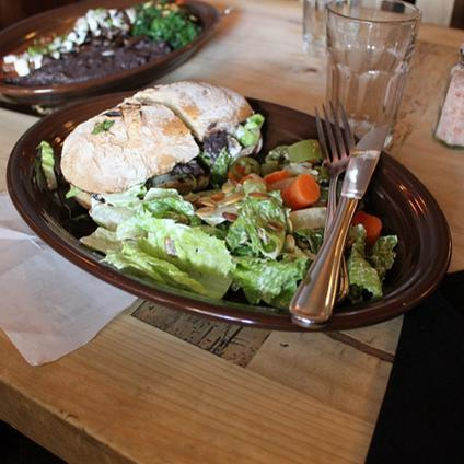
# want a target sample stimulus?
benchmark.get_stimulus(index=6)

A typically crucial piece of any brain dataset (and especially fMRI) are ‘regions of interests’ (ROIs). Our benchmark class here catalogues these automatically, and comes equipped with key functions that allow us to subset those parts of the brain data that correspond to each ROI.
benchmark.get_roi_structure(mode='global')
Level 0:ROI EVC, OTC, V1v, V1d, V2v, V2d, V3v, V3d, hV4, FFA-1, FFA-2
              OFA, EBA, FBA-1, FBA-2, OPA, PPA, VWFA-1, VWFA-2, OWFA
Level 1:SubjectID 1
Core Components
Admittedly, though, classes can be hard to work with. For that reason, let’s break down the 3 core components to any benchmark:
- Response Data: (BrainUnitID x StimulusID)
- Metadata: (BrainUnitID x …)
- Stimulus Data: (StimulusID x…)
response_data is the most important of these 3 components. In the case of a BrainBenchmark (like NSDBenchmark), the rows of this dataframe are the IDs of a target brain units (sometimes called “neuroids” by benchmarking platforms like BrainScore), the columns of this dataframe are the IDs of our target stimuli, and each cell is the response of a given brain unit (in this case voxels) to a target stimulus (in this case, a natural image).
Step 4: Alignment Procedure(s)
You have your benchmark data; you have your features. Now, it is time to put the two together. While many people refer to this step with many different names – correspondence test, encoding or decoding, representational similarity analysis – in DeepJuice, we tend to call it the “alignment procedure.” We use this term with the most general connotation possible, or at least the one we hope generalizes over the many different forms this particular step can take.
Why Multiple Metrics? A striking finding in recent work is that many qualitatively different DNN models – with different architectures, tasks, and training data – achieve comparably high alignment scores with human visual cortex. This relative parity suggests that standard alignment metrics may be capturing broad, shared structure rather than the specific computational principles that distinguish models. Using multiple metrics with different assumptions can help reveal whether apparent alignment reflects genuine correspondence or simply the flexibility of the linking procedure.
In the example below (which directly follows the analyses from
-
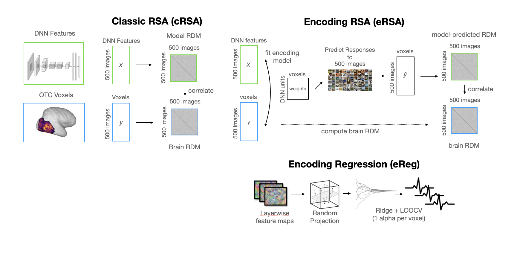
Classical RSA (cRSA): A paradigmatic representational similarity analysis that directly computes the representational geometry of the target brain and model data (using the Pearson distance), then directly compares the resultant representational dissimilarity matrices (RDMs) with no intermediate reweighting (again using the Pearson distance). This analysis assumes a fully-emergent fit between model and brain that weights all model features equally, and in this sense is one of the stricter tests of alignment one can use.
-
Encoding Regression (eReg): This alignment procedure unfurls in multiple steps. First, for computational efficiency and to control explicit degrees of freedom, we use a dimensionality reduction technique called sparse random projection to project each of our feature maps into a lower-dimensional space. This step relies on the Johnson-Lindenstrauss Lemma
, a theorem guaranteeing that points in a high-dimensional space can be embedded into a lower-dimensional space while approximately preserving pairwise distances. Crucially, the target dimension depends logarithmically on the number of samples (images), not the original feature dimension. After reducing the dimensionality of our feature space, we apply ridge regression to the reduced features. -
Encoding RSA (eRSA): Elsewhere developed as feature-reweighted RSA
, this alignment procedure is a way of taking the encoding models from the ridge regression procedure above, and using them to build RDMs. This procedure liberates our RSA from the assumption that all features must be weighted equally, and leverages the trimming and redistribution of feature importances done by the encoding model to give us a more explicitly brain-aligned representational geometry.
Below is a more detailed visual schematic of these methods:
Of course, scoring the alignment between a given model’s feature space and the brain doesn’t necessarily tell us all that we’d like to know. Once we’ve scored the alignment across many feature spaces from a single model (or from many models), we’d ideally like to know why certain feature spaces score higher than others.
There are obviously many theories for this, but in the example below, we’ll look at one increasingly popular candidate called effective dimensionality, which quantifies how the variance in a given feature space is distributed across its principal components. This metric has been linked to generalization performance in neural networks and the dimensionality of neural representations in the brain
Prepare Benchmark Data
The first thing we’ll need to do to be able to run our alignment procedure is to compute the target RDMs from our target brain data. If we’ve already specified ROIs in this data, we can compute these RDMs simply by passing an RDM function (i.e. a squareform distance metric) to a convenience function from our benchmark class.
from deepjuice.alignment import compute_rdm
benchmark.build_rdms(compute_rdm, method='pearson')
Score the Feature Maps
And now, in one grand swoop, we’re going to use our Benchmark() and our FeatureExtractor() to loop through all feature_maps and score them on the alignment procedures outlined above.
Define: get_benchmarking_results() + helpers
```python from deepjuice.alignment import get_scoring_method def effective_dimensionality(feature_map): # first, we define a GPU-capable PCA pca = TorchPCA(device='cuda:0') # then fit the PCA... pca.fit(feature_map) # then extract the eigenspectrum eigvals = pca.explained_variance_ # then return effective dimensionality (on CPU) return (eigvals.sum() ** 2 / (eigvals ** 2).sum()).item() def get_benchmarking_results(benchmark, feature_extractor, layer_index_offset = 0, metrics = ['cRSA','eReg','eRSA'], rdm_distance = 'pearson', rsa_distance = 'pearson', score_types = ['pearsonr'], stack_final_results = True, feature_map_stats = None, alpha_values = np.logspace(-1,5,7).tolist(), regression_means = True, device='auto'): # ... (full implementation in notebook) pass ```stats = {'effective_dimensionality': effective_dimensionality} # stats to compute over features
results = get_benchmarking_results(benchmark, feature_extractor, feature_map_stats = stats)
Parse Results (Scores)
The results you now have are comprehensive, but complicated: one score per feature map (layer) per ROI per subject per train-test split per metric. If you’re doing analyses across multiple models, you’ll then multiply these combinatorics even further with scores per model. Generally speaking – and while this choice comes with assumptions the field should probably start examining a bit more closely – most model-to-brain alignment procedures include the taking of a max over layers.
from deepjuice.benchmark import get_results_max

# variables over which we'll take the max:
max_over = ['model_layer','model_layer_index']

# all variables for which we want the max:
group_vars = ['metric', 'region', 'subj_id']

# criterion is the column in results that is used to select the maxs
get_results_max(results, 'score', group_vars, max_over,
                criterion={'cv_split': 'train'}, filters={'region': ['EVC','OTC']})
Step 5: Visualize your Results
So now, we have some results! What do you do with them? Contribute to the advancement of knowledge, ideally. But first! Let’s start with some plots, and a bit of analysis.
Import plotnine (ggplot)
```python from plotnine import * # python's ggplot import plotnine.options as ggplot_opts ```# these are the results columns we'll need for plot
target_cols = ['model_layer_index','model_layer','region',
'subj_id','cv_split','score','effective_dimensionality']
target_region = 'OTC' # first, we'll look at occipitotemporal cortex
# we subset our results for our region of interest:
plot_data = results.query('region == @target_region')
# here, we convert model_layer_index into a relative depth (0 to 1)
plot_data['model_layer_depth'] = (plot_data['model_layer_index'] /
plot_data['model_layer_index'].max())
ggplot_opts.figure_size = (10,4) # set figure size
# this defines our plotting geometry / aesthetics
mapping = {'x': 'model_layer_depth', 'y': 'score',
'group': 'cv_split', 'color': 'cv_split'}
# and now, we invoke python's ggplot via plotnine!
(ggplot(plot_data, aes(**mapping)) + geom_line() +
facet_wrap('~metric')+ theme_bw()).draw()
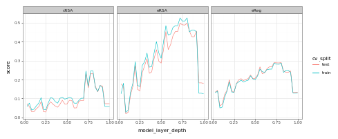
Here, we see that (pretty much up until the last layers) our scores for occipitotemporal cortex (OTC) tend to increase. (The dropoff in the last layers is a byproduct of the fact that we’re working with a self-supervised model in this demo, and these layers correspond to the projection head of the model – whose features aren’t always particularly useful or predictive). Now, let’s look at the same plot with the addition of early visual cortex (EVC):
target_region = ['EVC','OTC'] # now, we add early visual cortex

plot_data = results.query('region == @target_region')
plot_data['model_layer_depth'] = (plot_data['model_layer_index'] /
                                  plot_data['model_layer_index'].max())

mapping = {'x': 'model_layer_depth', 'y': 'score',
           'group': 'region', 'color': 'cv_split'}

mapping['linetype'] = 'region' # for comparison

(ggplot(plot_data, aes(**mapping)) + geom_line() +
 facet_grid('cv_split~metric')+ theme_bw()).draw()
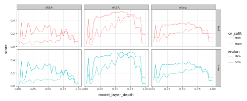
Here, we see that predictions for EVC tend to peak earlier than they do for late-stage visual cortex (OTC) – though not by as much as you might otherwise expect… (While we don’t have time to go too deeply into this result here, if you’re interested in following-up on this, a good place to start would be to consider receptive field sizes!)
Finally, let’s look at the relationship between effective dimensionality and score across layers:
target_region = 'OTC' # just occipitotemporal cortex again

# we subset our results for our region of interest:
plot_data = results.query('region == @target_region')

mapping = {'x': 'effective_dimensionality', 'y': 'score',
           'group': 'cv_split', 'color': 'cv_split'}

(ggplot(plot_data, aes(**mapping)) + geom_point() +
 geom_smooth(method='lm') + facet_wrap('~metric')+ theme_bw()).draw()
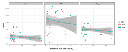
Here, we see effectively no relationship. Why? Well, the reasons are complex, and full enumeration thereof is beyond the scope of this tutorial – but one function it serves here, at least, is to highlight that downstream alignment (at least to this very popular visual brain data) is not always 1:1 with what you might expect from the effective “degrees of freedom” inherent to the feature space of a candidate model.
Enter Now the LLMs
Cross-Modal Brain Alignment
Recent success predicting human ventral visual system responses from large language model (LLM) representations of image captions has sparked renewed interest in the possibility that high-level visual representations are “aligned to language”
What might explain this convergence? One hypothesis, articulated in the “Platonic Representation Hypothesis”
Recent work has begun to dissect this question more carefully.
These findings raise important questions: Which aspects of representation are shared across modalities, and which are modality-specific? In this chapter, we demonstrate techniques for probing cross-modal alignment using the same NSD data from Chapter 1.
In this section, we walk through an example of cross-modal alignment using the same subset of the NSD dataset as before. Language models can be loaded through DeepJuice, but for demonstration purposes, we load a sentence transformer model from Huggingface directly.
from transformers import AutoTokenizer, AutoModel

model_uid = 'sentence-transformers/all-MiniLM-L6-v2'
model = AutoModel.from_pretrained(model_uid)
tokenizer = AutoTokenizer.from_pretrained(model_uid)
Each of the images in the NSD dataset is actually an image from the COCO dataset, and each image in the COCO dataset comes with 5-6 human annotations (captions). By default (at least in the NSD metadata), the COCO captions are stored as stringified lists.
from deepjuice.structural import flatten_nested_list # utility for list flattening

all_captions = benchmark.stimulus_data.coco_captions.tolist() # list of strings

# the listification and flattening of our 5 captions per image into one big list:
captions = flatten_nested_list([eval(captions)[:5] for captions in all_captions])

assert(len(captions) == 1000 * 5) # assertion to ensure each image has 5 captions

np.random.choice(captions, 5).tolist() # a sample showing what our captions look like
['Two children standing next to a yellow fire hydrant',
 'Skier skiing down a hill near a guard rail ',
 'A suitcase on a bed with a cat sitting inside of it.',
 'A man riding a surfboard on top of a wave in the ocean.',
 'a train being worked on in a train manufacturer']
Pretty much everything from here forward matches exactly the benchmarking procedure above! In this example, we’ll calculate the cRSA, SRPR, and eRSA score for our target set of language embeddings, saving the results for two key ROIs (early visual and occipitotemporal cortex) for the purposes of downstream comparison:
target_region = ['EVC','OTC'] # early and late visual cortex

plot_data = results.copy()[results['cv_split'] == 'test'].query('region == @target_region')

# this gives us a "depth ratio" from 0 (earliest layer) to 1 (latest)
plot_data['model_layer_depth'] = (plot_data['model_layer_index'] /
                                  plot_data['model_layer_index'].max())

# putting our metrics in order as a factor (Categorical)
plot_data['metric'] = pd.Categorical(plot_data['metric'],
                                     categories=['cRSA','eReg','eRSA'])

from plotnine import * # ggplot functionality

# define an aesthetic mapping for ggplot call:
mapping = {'x': 'model_layer_depth', 'y': 'score',
           'group': 'region', 'color': 'region'}

(ggplot(plot_data, aes(**mapping)) +
 geom_line(size=2) +facet_wrap('~metric')+ theme_bw()).draw()
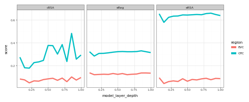
Notice here that language models do exceptionally well in predicting late-stage visual cortex (OTC), but not so well in predicting early visual cortex (EVC)! This is a nice sanity check, and suggests the high scores in late-stage visual cortex are indeed the result of shared representational structure, as opposed to a mere statistical fluke.
Vector-Semantic Mapping
Hypothesis-driven interpretation via “relative representations”
The use of deep neural network models to predict brain and behavioral phenomena typically involves procedures that operate over dense, high-dimensional vectors whose underlying structure is largely opaque. However accurate these procedures may be in terms of raw predictive power, this ambiguity leaves open fundamental questions about what drives the measured correspondence between model and brain.
The Core Idea:
“We propose the latent similarity between each sample and a fixed set of anchors as an alternative data representation.”
This move toward interpretable alignment allows us to bridge the gap between opaque neural features and grounded semantic concepts.
Anchor Points as a Coordinate System: Think of this as defining a new coordinate system where each axis is “similarity to anchor X.” If we choose our anchors wisely – using natural language queries that correspond to interpretable concepts – then the resulting representation is both lower-dimensional and human-readable. Each dimension has a clear meaning: “how much does this image resemble [query]?”
Connection to Zero-Shot Classification: This technique is closely related to how CLIP performs zero-shot classification
We will use this technique to probe what kinds of semantic information (expressible in natural language) drives the predictive power of LLMs for visual brain activity.
Classification Warmup Example
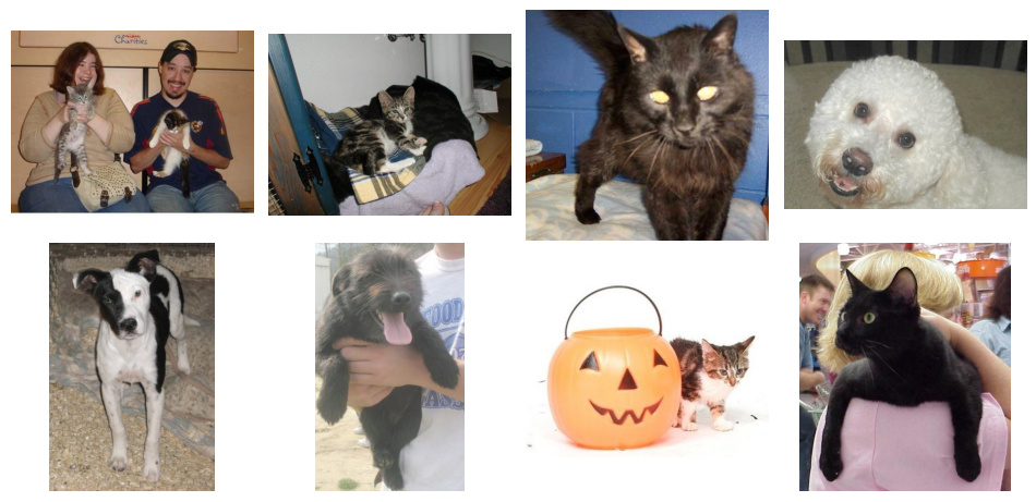
Below is a schematic of the basic idea of vector-semantic mapping using relative representations, applied to the binary classification task of cat and dog images based on the embeddings of a CLIP-like vision encoder.

Relative representations are a way to quickly warp high-dimensional embeddings into new (lower-dimensional) coordinates defined by a set of custom queries (also called anchor points).
device = get_available_device()
print(f"Using device: {device}")

model, _, preprocess = open_clip.create_model_and_transforms('ViT-B-16-SigLIP', pretrained='webli')
model = model.eval().to(device)

tokenizer = open_clip.get_tokenizer('ViT-B-16-SigLIP')

hf_data = load_dataset('cats_vs_dogs', cache_dir='../datasets')['train']
image_dataset = ImageDataset(hf_data, preprocess, image_key='image', label_key='labels')

image_loader = DataLoader(image_dataset, batch_size=64, shuffle=True)
Using device: cuda
print('A sample of dog and cat images:')
image_dataset.show_sample(n=8, nrow=2, figsize=(10, 5))
Binary Classification with Full Embeddings
We now have the dataset we can use to perform our binary classification task. First, we’ll split our embeddings (and their associated category labels) into train and test sets…
embeds = embeds.to('cpu') # move to cpu, just in case

# use odd / even indices for train / test split:
train_X, test_X = embeds[0::2, :], embeds[1::2, :]
train_y, test_y = labels[0::2], labels[1::2]
… then, we fit our classifier (a regularized logistic regression with internal cross-validation to select the regularization parameter, alpha).
clf = RidgeClassifierCV(alphas=[1e-3, 1e-2, 1e-1, 1, 1e2, 1e3])
clf.fit(train_X, train_y)

print('Binary Classification Accuracy:')
print(clf.score(test_X, test_y))
Binary Classification Accuracy:
0.9976078598889363
Classification with Relative Representations
Now we arrive at the key technique. Instead of classifying over the full 768-dimensional embedding space, we project images into a lower-dimensional space defined by similarity to language queries. As
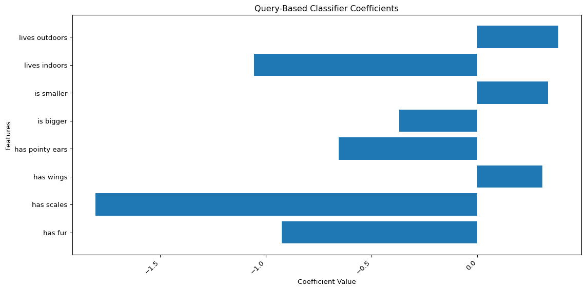
query_strings = ['has fur', 'has scales', 'has wings', 'has pointy ears',
                 'is bigger', 'is smaller', 'lives indoors', 'lives outdoors']

query_embeds = get_query_embeds(query_strings)
print('Query Embeddings Shape:', query_embeds.shape)
Query Embeddings Shape: torch.Size([8, 768])
After embedding our language queries, we compute their cosine similarity to each image embedding. But now, instead of using softmax over similarity scores, we use them as features in a regularized classifier.
similarity = embeds @ query_embeds.T

X_train, X_test = similarity[0::2, :], similarity[1::2, :]
y_train, y_test = labels[0::2], labels[1::2]
clf = RidgeClassifierCV(alphas=[1e-3, 1e-2, 1e-1, 1, 1e2, 1e3])
clf.fit(X_train, y_train)

print('Binary Classification Accuracy:')
print(clf.score(X_test, y_test))
Binary Classification Accuracy:
0.9119179837676207
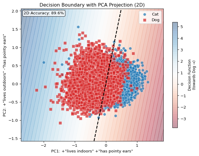
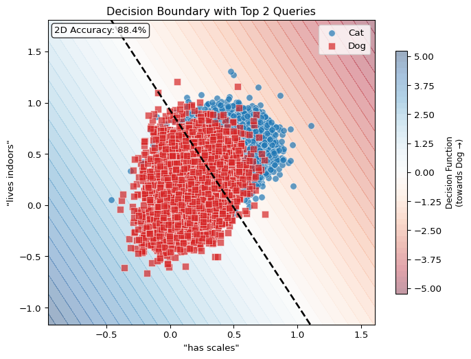
Notice now that the number of coefficients in our classifier corresponds 1:1 with the number of queries we made… And because our queries were made with natural language, we can actually interpret these coefficients in terms of their ‘importance’ in determining the correct label!
Brain Alignment with Relative Representations

The classification example above demonstrates that relative representations can preserve task-relevant structure while providing interpretable coefficients. But the more topic-relevant question motivating the use of this technique in this tutorial is: Can we use relative representations to understand what drives model-brain alignment?
When we fit a standard encoding model, we learn weights over thousands of opaque features. We can measure alignment, but we cannot easily interpret why certain images are predicted well or poorly. Relative representations offer a path forward: by projecting both model features and brain activity into a shared space defined by interpretable language queries, we can ask which semantic dimensions are most important for predicting neural responses.
This is a form of hypothesis-driven alignment analysis. Rather than asking “how well does this model predict the brain?” we ask “which semantic concepts, expressible in language, mediate the correspondence between model and brain?”
Defining the Semantic Basis
The power of relative representations depends critically on the choice of anchor points. In
Define hypothesized semantic queries (73 anchor points)
```python prompt_options = {} # initialize a dictionary for our query options (by categories, for clarity) prompt_options['camera'] = ['a picture', 'a drawing', 'a rendering'] prompt_options['quality'] = ['high resolution', 'low resolution', 'high quality', 'low quality', 'dark', 'bright', 'cluttered', 'clean', 'happy', 'sad', 'colorful', 'black-and-white', 'professional', 'candid', 'artistic'] prompt_options['agent'] = ['a person', 'a group of people', 'an animal', 'a group of animals'] prompt_options['object'] = ['an object', 'a group of objects', 'furniture', 'food', 'a plant', 'plants', 'a vehicle', 'vehicles'] prompt_options['adjective'] = ['big','small','boxy','curvy','rural', 'urban', 'slow', 'fast', 'dangerous', 'safe', 'indoors','outdoors'] prompt_options['places'] = ['work', 'a desk', 'a room', 'a building', 'a city', 'a park', 'a field', 'a beach', 'the water', 'the sky', 'the snow', 'the desert', 'the mountains'] prompt_options['time'] = ['in the morning', 'at night', 'during the day', 'in winter', 'in spring', 'in summer', 'in autumn'] prompt_options['action'] = ['playing', 'working', 'fighting', 'dancing', 'jumping', 'sitting', 'standing', 'running', 'walking', 'swimming', 'flying'] # flatten our categorized query options into a single list all_prompts = list(chain(*prompt_options.values())) print('Number of prompts (hypothesized anchor points): {}'.format(len(all_prompts))) ```Number of prompts (hypothesized anchor points): 73
To see how well these queries define the representational alignment of our vision model to the visual brain data, we simply need again to compute the similarity of each query to each image embedding, then fit a regression over the resultant similarity scores.
query_embeds = get_query_embeds(all_prompts)
print('Shape of query embeddings:', [el for el in query_embeds.shape])

image_query_sims = image_embeds @ query_embeds.T
print('Shape of similarity matrix:', [el for el in image_query_sims.shape])
Shape of query embeddings: [73, 768]
Shape of similarity matrix: [1000, 73]
type_label = 'Regression on Hypothesized Query Similarities'
hypothesis_query_results = compute_alignment(image_query_sims, type_label)

print('Scoresheet for our hypothesized query regression:')
hypothesis_query_results['scoresheet']
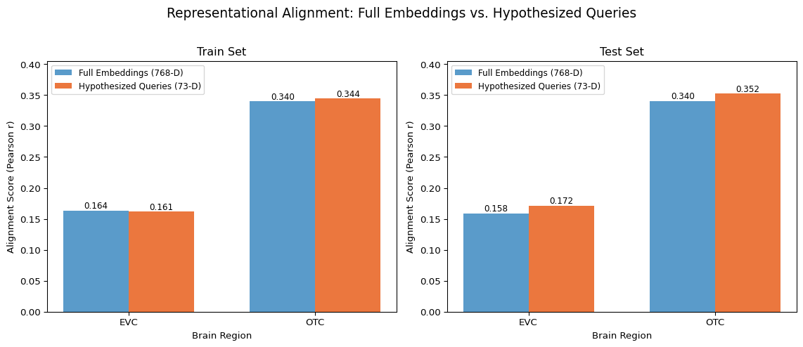
Dimensionality reduction: 768 -> 73 (9.5% of original)
EVC: 108.3% performance with 90.5% fewer dimensions
OTC: 103.5% performance with 90.5% fewer dimensions
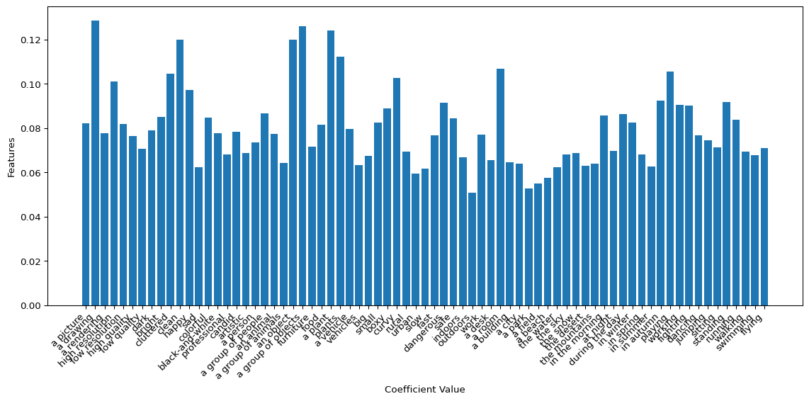
And so – What do we see here? Well, first and foremost we see that with only 73 queries (73 total predictors, 73 dimensions) we can recover the full predictive power of the underlying 768-dimensional embedding space!
And now, taking the mean absolute value of the coefficients for each query, we can see which of our 73 dimensions weighed most on our downstream brain data prediction!
Visualization: Coverage of the Manifold
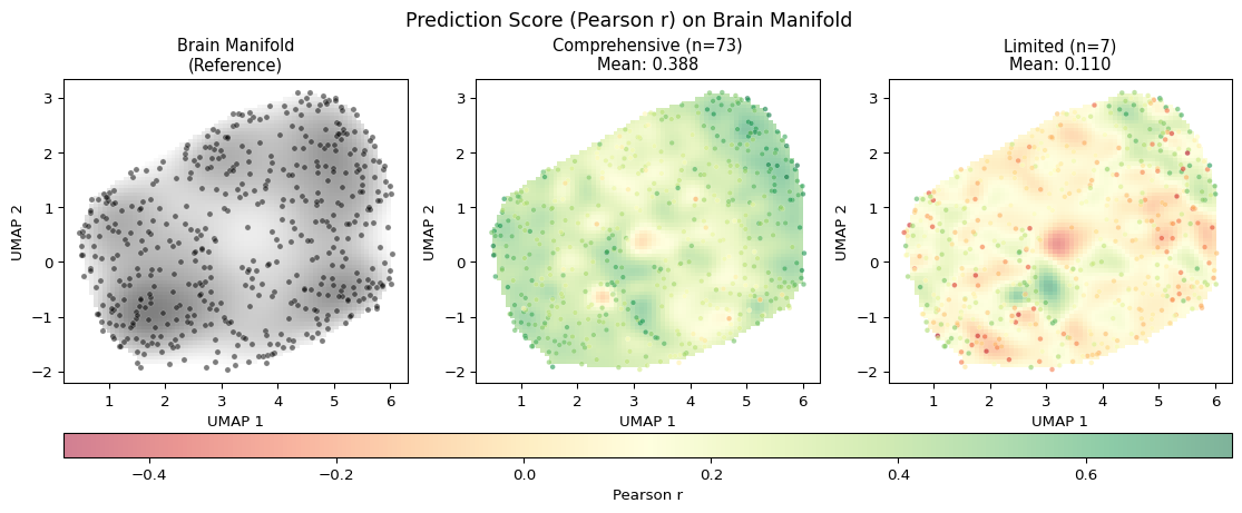
To better understand how our query-based representations relate to the brain representational space, we can visualize both spaces using dimensionality reduction techniques. These visualizations help illustrate:
- How query similarities “cover” the brain representational space
- The geometric correspondence between query and brain spaces
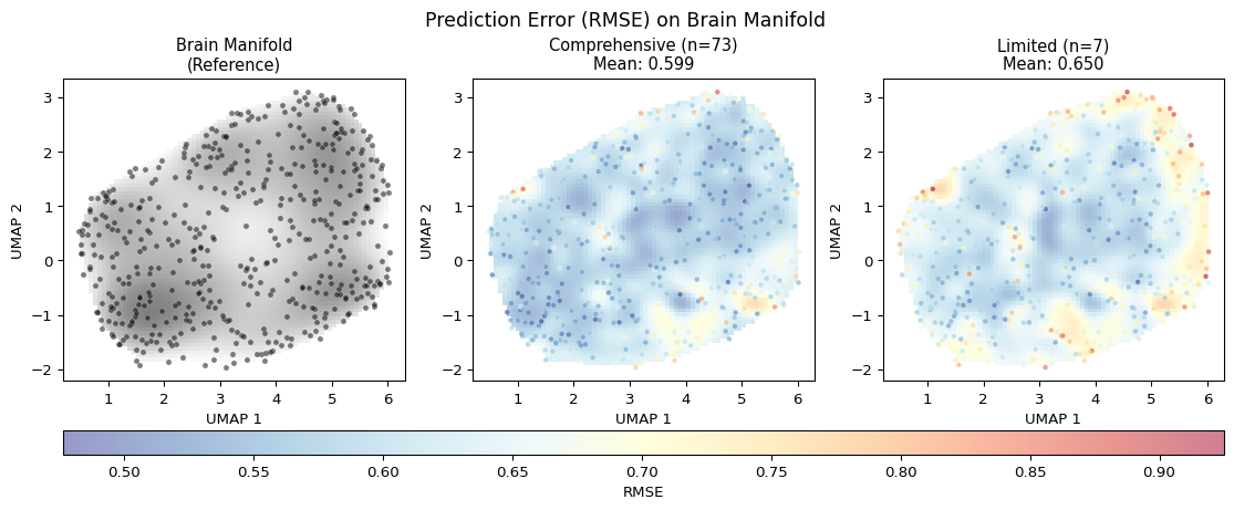
Prediction Error on the Brain Manifold
A key insight from
Comparison: Random vs. Hypothesized Queries
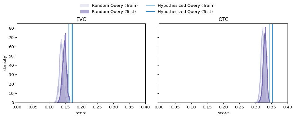
… what do we find? On the one hand, our hypothesized queries do indeed consistently (uniformly, in fact) outperform the random queries of the same size…
… On the other hand, they do so by a much smaller margin than you might expect if our hypothesized queries were indeed exceptional in a deeply meaningful way…
Further interpretation of these results is… an active area of research! And as such (albeit very much a regrettable cliffhanger), a topic we leave for you as food-for-thought. So as not to leave you fully hanging, though, here’s some questions we’ve been pondering:
- What do these results tell us (if anything) about the nature of cross-modal alignment between language models and the visual brain? Is it a fluke? Or more evidence of ‘platonic’ representational structure?
- By what mechanism could the random queries perform as well as they do?
- What, if anything, might this finding have to do with effective dimensionality?
- What, if anything, could we do to improve the hypothesized queries?
- Is there more variance left to capture? If so, how much, and with what kinds of queries?
Conclusion
Our tutorial has now taken us on a somewhat whirlwind tour through the core methods of representational alignment research in computational cognitive neuroscience: extracting features from deep neural networks, comparing them to brain activity using multiple metrics (RSA and encoding models), and probing cross-modal alignment between vision and language representations.
A Note on Scope: Throughout this tutorial, we have demonstrated these methods on a small number of example models. The findings from any single model (or handful of models) should be interpreted cautiously – the real power of this approach emerges when applied systematically across many models, as in
Key Takeaways:
-
Different metrics reveal different aspects of alignment: Classical RSA provides a strict test of emergent geometric correspondence, while encoding models allow flexible feature reweighting. The choice of metric embodies assumptions about what constitutes a “good” match between model and brain.
-
Many different models achieve comparable alignment: A striking finding here and in the broader literature is that qualitatively different models (even those trained on entirely different modalities of data) often achieve similar brain-predictivity scores. This parity – not visible when testing single models – motivates the multi-model, many-metric (but single pipeline!) approach demonstrated here.
-
Cross-modal alignment raises deep questions: The fact that language models can predict visual cortex activity challenges simple modular accounts of brain organization. Whether this reflects genuine shared representations or statistical artifacts remains actively investigated.
-
Interpretability is a moving target: The interpretability of DNNs is a moving target, circumscribed by every choice in our experimental pipelines: the data we use as probes, the model populations we sample to assess divergence, and the metrics we use to quantify greater and lesser alignment to the downstream brain and behavioral phenomena that are our ultimate targets.
Looking Forward: The broader vision of NeuroAI
Feel free to reuse, remix, and extend this code. For questions or suggestions, please reach out via the associated GitHub repository.
Related Software
This tutorial uses DeepJuice for high-throughput neural network analysis. We gratefully acknowledge the broader ecosystem of tools for representational alignment research:
Neural Benchmarking Platforms:
-
Brain-Score - Integrative benchmarks for brain-like AI
- Net2Brain - Toolbox for comparing DNNs to brain data
Representational Similarity and Alignment:
- RSAToolbox - Representational Similarity Analysis in Python
- NetRep - Metrics for comparing neural network representations
- Similarity - Repository of similarity measures
- Himalaya - Fast kernel methods for encoding models (Gallant Lab)