NLDisco: A Pipeline for Interpretable Neural Latent Discovery

Large-scale neural recordings contain rich structure, but identifying the underlying representations remains difficult without tools that produce interpretable, neuron-level features. This tutorial introduces NLDisco (Neural Latent Discovery pipeline), which uses sparse encoder–decoder (SED) models to identify meaningful latent dimensions that correspond to specific behavioural or environmental variables.

Goal

Discover interpretable latents (i.e., features) in high-dimensional neural data.

Terminology

• Neural / Neuronal: Refers to biological neurons. Distinguished from model neurons (see below).
• Units: Putative biological neurons - the output from spikesorting extracellular electrophysiological data.
• Model neurons: Neurons in a neural network model (aka latents)
• Features: Interpretable latents (latent dimensions that align with meaningful behavioural or environmental variables)

Method overview

Sparse Autoencoders

Motivated by successful applications of sparse dictionary learning in AI mechanistic interpretability , NLDisco trains overcomplete sparse encoder-decoder (SED) models to reconstruct neural activity based on a set of sparsely active dictionary elements (i.e. latents), implemented as hidden layer neurons. In the figure below, this is illustrated as reconstructing target neural activity \(z\) from input neural activity \(y\) via dictionary elements \(d\). Sparsity in the latent space encourages a monosemantic dictionary, where each hidden layer neuron corresponds to a single neural representation that can be judged for interpretability, making SEDs a simple but effective tool for neural latent discovery.

For example, in a monkey reaching task, you might find a latent that becomes active mainly during high-velocity hand movements, and this latent can then be traced back to the subset of biological neurons whose activity consistently drives it.

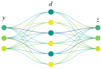
These SEDs can be configured as autoencoders (SAEs) if the target for \(z\) is \(y\) (e.g. M1 activity based on M1 activity), or as transcoders if the target for \(z\) is dependent on or related to \(y\) (e.g. M1 activity based on M2 activity, or M1 activity on day 2 based on M1 activity on day 1). In this tutorial, we will work exclusively with the autoencoder variant, specifically Matryoshka SAEs (MSAEs).

Matryoshka Architecture

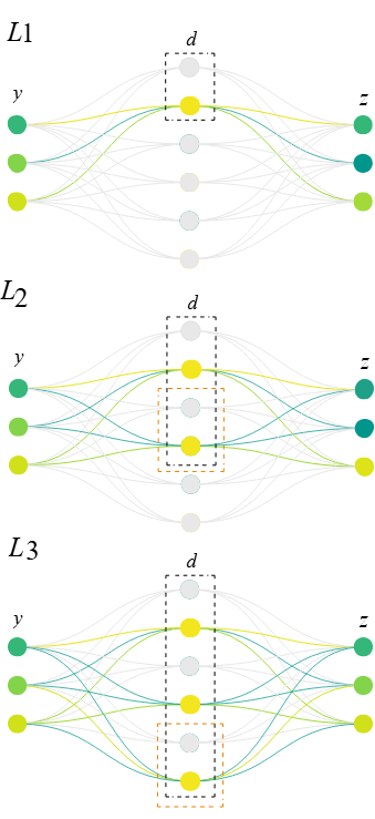
The Matryoshka architecture segments the latent space into multiple levels, each of which attempts a full reconstruction of the target neural activity . In the figure below, black boxes indicate the latents (model neurons) involved in a given level, while light-red boxes indicate additional latents recruited at lower levels. A top-\(k\) selection is used to choose which latents to recruit for reconstruction at each level (yellow neuron within each light-red box - \(k=1\) for each level in this example).

This nested arrangement is motivated by the idea that multi-scale feature learning can mitigate “feature absorption” (a common issue where a more specific feature subsumes a portion of a more general feature), allowing both coarse and detailed representations to emerge simultaneously.

• Latents in the highest level (\(L_1\)) typically correspond to broad, high-level features (e.g., a round object),
• Latents exclusive to the lowest level (\(L_3\)) often correspond to more specific, fine-grained features (e.g., a basketball)

Code

The code for the full tutorial showcasing the NLDisco pipeline can be accessed here. The notebook contains step-by-step instructions and descriptions for each stage of the pipeline. It follows this structure:

1. Load and prepare data - Load neural spike data from the Churchland MC_Maze dataset (center-out reaching task with motor cortex recordings) , pre-process into binned spike counts, and prepare behavioural/environmental metadata variables (hand position, velocity, maze conditions, etc.) for later feature interpretation.
2. Train models - Train MSAE models to reconstruct neural activity patterns. Multiple instances are trained with identical configurations for comparison to ensure convergence, with hyperparameters for sparsity and reconstruction quality. Validation checks examine decoder weight distributions, sparsity levels (L0), and reconstruction performance.
3. Save or load the model activations - Save trained SAE latent activations for efficient reuse, or load pre-computed activations to skip directly to feature interpretation.
4. Find features - Automatically map latents to behavioural and environmental metadata by computing selectivity scores that measure how strongly each latent activates during specific conditions (e.g., particular maze configurations, velocity ranges). Use an interactive dashboard to explore promising latent-metadata mappings and identify which biological neurons contribute most to interpretable features.